Training a Single Neuron to Convert Celsius to Fahrenheit
2026-11-17 · 6 min read
The idea of this project is to work as an introduction to Machine Learning. ML is interesting because it changes paradigm from “imperative programing” where you indicate each step to reach the desired output, to “Declarative programing” where we only will indicate the final state and the system figures out how to get there. In this project we will train a neuron to convert Celsius to Fahrenheit with TensorFlow
Dependencies
Before we can begin training any model, we first need three things, Import the dependences, a data set to train the model on, and we need to define the model. Our first step is to import TensorFlow to define and train the model, and NumPy and matplotlib to graph analyze the performance.
import tensorflow as tf

import numpy as np

import matplotlib.pyplot as plt
Dataset Generation
before we can create the data set to train the model, we first must define how we are going to train it. We can choose from supervised, unsupervised training, or a hybrid approach.
Supervised training
- This is where we feed the model labeled data with known correct answers. The goal is for the model to adjust, until it can predict the known correct output based on the input.
Unsupervised Training
- We give the model unlabeled data and it finds its own meaning in the data. In this type of training there are no correct answers. The goal here is to find hidden relationships in data.
Hybrid
- There are multiple ways to mix these models, for example: Semi supervised, where a small part of the data is labeled and the rest are unlabeled.
In the case of our project we are going to provide the model an array of values in Celsius(Features/inputs) and an array of the answer in Fahrenheit(Labels/Targets), meaning we are supervising the training.
# Celsius numpy array with an explicitly defined data type of float.
celsius_q = np.array([-40, -10, 0, 8, 15, 22, 38], dtype=float)

# Fahrenheit numpy array with explictly defined data type of float.
fahrenheit_a = np.array([-40, 14, 32, 46, 59, 72, 100], dtype=float)
Model Definition (1-Neuron ANN)
In the following section we are going to define the models structure. The structures include how many neurons will the model contain, how many layers of neurons, how the neurons will be connected to each other, and the expected input.
model = tf.keras.Sequential(
    [tf.keras.layers.Dense(units=1, input_shape=[1])])
In TensorFlow code, tf is an alias for the TensorFlow library.
Keras is an abstraction layer that sits on top of the raw TensorFlow mechanics and handles graph building, gradients, and so on. This is the part that makes it beginner-friendly.
Sequential is a class that defines the stack of layers of neurons, in other words, it defines the shape and size of the model. A Sequential model moves in only one direction: forward.
tf.keras.Sequential([])
Inside the square brackets:
- layers: a module inside Keras containing layer types.
- Dense: a layer type where every input connects to every neuron.
- units=1 : defines the neurons in this layer.
- input_shape=[1] : defines the expected input into the model.
tf.keras.layers.Dense(units=1, input_shape=[1])
All of this comes together to define the model’s structure.
Compilation
Compilation here isn’t the same as in tradicional programing. Compilation in kares means preparing and configuring the model for training. Here we tell Kares:
- How to measure how wrong a prediction is.
- Defining how the algorithm should adjust its weights
- Optionally Stat you want to display while training
model.compile(loss='mean_squared_error', optimizer=tf.keras.optimizers.Adam(0.1))
The compile method tells Keras to build and configure model using the arguments previously defined. The arguments:
- loss=’mean_squared_error’ : Defines the error measurement. It squares the difference between predicted and actual values, then averages those squared errors.
- optimizers : A submodule of Keras containing the training algorithms.
- Adam A class implementing the Adam training algorithm.
- Adam(0.1) Defines how aggressive the adjustments to the weights will be. The value passed in is the learning rate.
Training
This is where we will train the model, define the inputs, outputs and the number of times the model will iterate through the training data.
history = model.fit(celsius_q, fahrenheit_a, epochs=500, verbose=True)
The fit method makes the model iterate through the training loop. The Arguments fed into the fit method define the following:
- Epochs: Define how many times the model will pass through the data sets
- Verbose: Controls whether the training progress get printed to the screen.
- Features: The inputs fed into the model. In this case celsius_q
- Labels: The expected outputs the model learns from. In This case fahrenheit_a
Data Output and Visualization
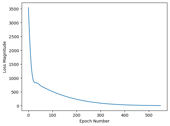
After the model finished training we can print out the wights and bias of a single neuron model. Additionally i graphed the change in loss with matplotlib.
print("Finished training the model")

print(f"Weight: {model.get_weights()}") # Should be ~1.8

print(f"Bias: {model.get_weights()[1]}") # Should be ~32
Change in loss
Conclusion
A single neuron learns the inherent rule of converting Celsius to Fahrenheit by taking its default weight and bias and adjusting them using Adam, guided by the magnitude of the loss, in other words, how wrong the output was.
Consider the basic formula inside a neuron: Y = WX + B, where Y is the result and X is the input. Compare that with the conversion formula, F = 1.8C + 32. Both are linear functions with the same shape: an input multiplied by a constant, plus another constant.
This is exactly why the model can learn this task at all. There is only one set of weight and bias values that maps Celsius to Fahrenheit correctly, so as training progresses, the only way to reduce the loss is for the weight to converge on 1.8 and the bias to converge on 32. If the model moved anywhere else, the loss would not decrease.
So after 500 iterations over the training set, the model has effectively rediscovered the conversion formula on its own, the weight settles near 1.8, the bias near 32, and the single neuron behaves just like F = 1.8C + 32.